Introduction
Before we dive into the next steps, let’s rewind and catch up on the progress so far. By the end of week 3, I wrapped up dataset collection and data preprocessing, making the data primed and ready for model training.
The week 4 started with me trying to figure out which model would be the best: LSTMs, CNNs, or a combination of both. Additionally, if using LSTMs, should it be bidirectional or unidirectional? I decided to set aside the chaos and just start coding one to see where it goes.
LSTMs
Since the data consists of commercial features where temporal features are of utmost priority, I decided to start with LSTMs.
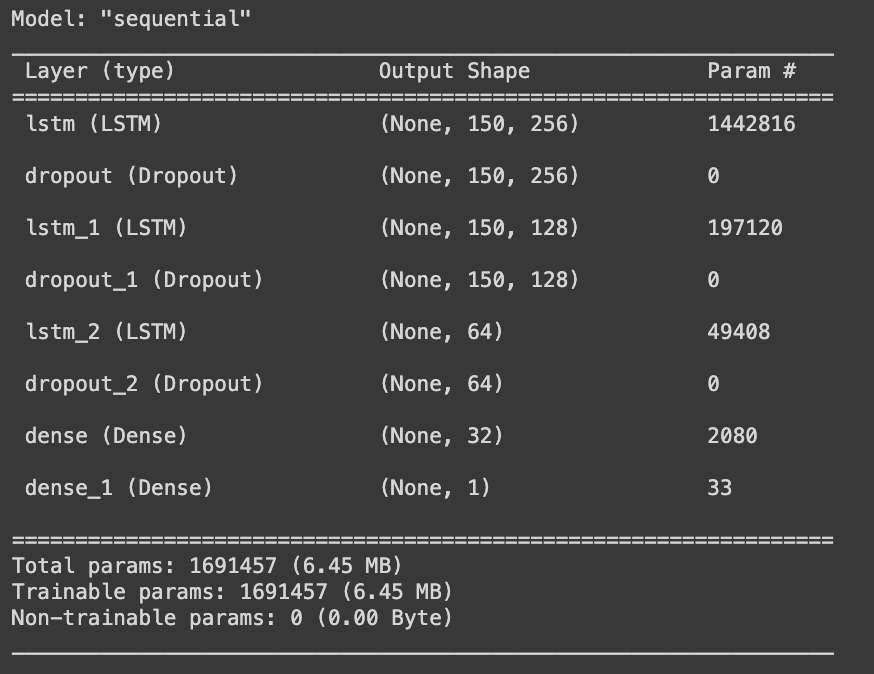
The unidirectional LSTM model consists of three LSTM layers, each followed by a dropout layer with a rate of 0.5 to ensure that the weights get generalized. The first two LSTM layers return a complete sequence of outputs, while the third LSTM layer returns only the output of the last time step. The LSTM layers are followed by two dense layers, which finally result in a single output value. The sigmoid activation function ensures that the final output is a value between 0 and 1, making it suitable for binary classification tasks like ours.
The model architecture of the unidirectional LSTMs is as shown:
Though unidirectional LSTMs are effective for sequential tasks, they do have limitations. They process sequences in only one direction, meaning at each time step, the model can access only past context, not future context.
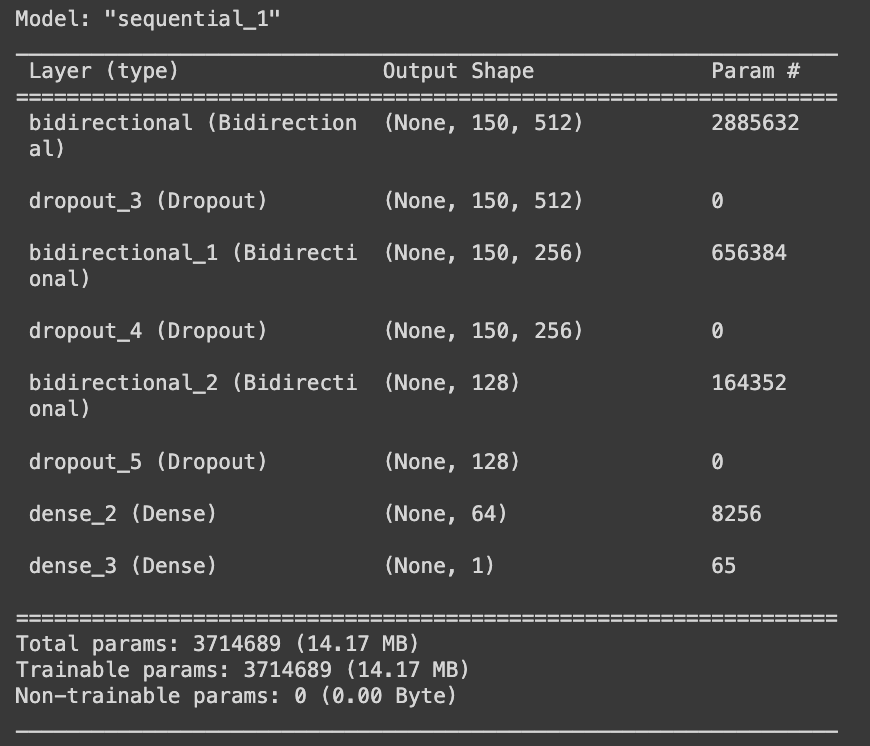
However, in scenarios like commercial videos that often start with a narrative and end with brand promotion, both past and future dependencies are crucial. To address this, I implemented a bidirectional LSTM model which takes both past and future features into account while training. I maintained a similar architecture to the unidirectional LSTM model but replaced the LSTM layers with bidirectional LSTM layers.
The architecture of the bidirectional LSTMs model is as follows:
CNNs
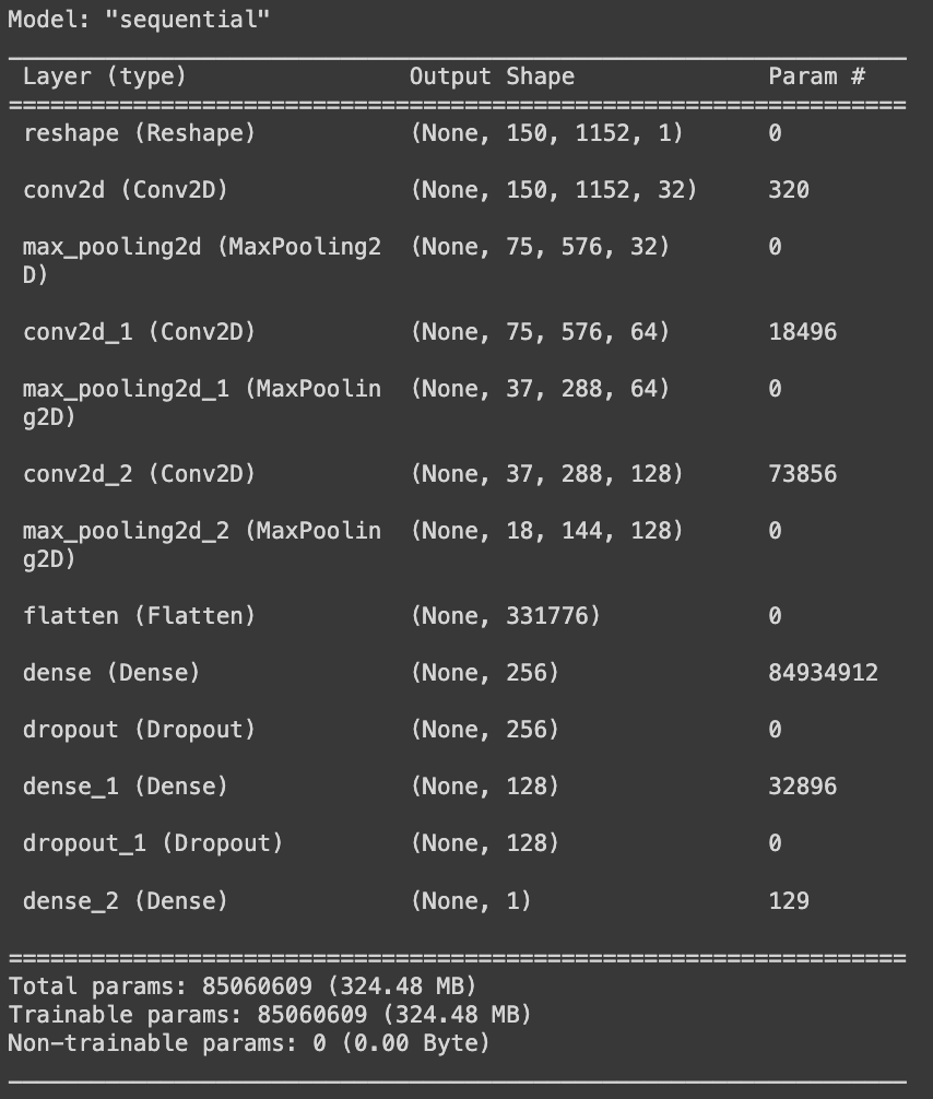
Considering the importance of both temporal and spatial features in commercial videos, I implemented a CNN model. This is the largest model I have implemented so far for this project, with over 85 million trainable parameters.
The CNNs model includes three convolutional layers:
- First with 32 filters
- Second with 64 filters
- And the third with 128 filters
Each of these layers use a 3x3 kernel size and ReLU activation function, ensuring feature extraction while preserving spatial information through padding. Max pooling layers follow each convolution to downsample the feature maps, enhancing computational efficiency and capturing dominant features. The flattened output is then fed into two dense layers with 256 and 128 units respectively, utilizing ReLU activation and dropout for regularization. The final dense layer with a sigmoid activation outputs a single probability value, suitable for binary classification tasks like commercial/no-commercial one.
The CNNs model architecture is as shown:
Other Models
I also implemented a CNNs+LSTMs model and a Transformers model. The architecture of both of these models is quite extensive so I am not adding it here. You can find their architectures here.
Results
| Model | Accuracy | True Positives | False Positives | True Negatives | False Negatives |
|---|---|---|---|---|---|
| Unidirectional LSTMs | 96.28% | 628 | 30 | 667 | 20 |
| Bidirectional LSTMs | 97.1% | 648 | 10 | 652 | 35 |
| CNNs | 93.97% | 623 | 35 | 646 | 41 |
| LSTMs+CNNs | 54.57% | 146 | 512 | 588 | 99 |
| Transformers | 96.05% | 640 | 18 | 652 | 35 |
From the results, it is clear that the LSTM models gave the best accuracy.
Deciding the Final Model
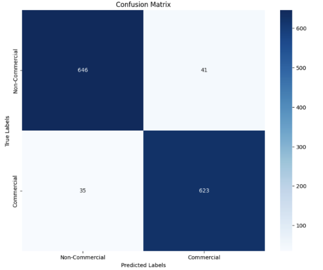
Although the best accuracy is given by LSTM model but it turns out that that TIDL doesn’t support LSTM layers. So, I will be going ahead with the CNNs model.
The confusion matrix of this model is as shown:
But, what is TIDL?
TIDL is “Texas Instruments” deep learning ecosystem which can be used to import networks trained to solve problems like classification, detection and segmentation and execute the networks for inference on Jacinto7 SoC exercising the C7x/MMA cores.
I will discuss more on it in the next Blog.
So, stay tuned!!
Thanks for reading the Blog.
Code of all these models can be found in this Link.