Introduction

The week started with me downloading the complete dataset again. Why? Didn’t I download it in week 0-1?

What happened is that I was downloading the dataset in shards and then appending the downloaded features into the same file. This process involves loading the already saved features from a .pkl file, appending the new features into the loaded features, and then saving it back into the same file. During one of these processes, the program loaded the features, appended them in the program, and while saving, the kernel crashed due to memory overflow. AHHH!!

My file became corrupted, and I was not able to open it, so I had to download the complete dataset again. This took me two days that I could have spent on dataset preprocessing.

Now, the dataset is downloaded. Let’s see its dimensions.

The shape of the different features is as shown:

commercialRgb : [4364][119-300][1024]
commercialAudio : [4364][119-300][128]
nonCommercialRgb : [4600][109-301][1024]
nonCommercialAudio : [4600][109-301][128]

What do the different dimensions of the features represent?

The first dimension represents the number of videos whose features are extracted. This is why this is constant for both audio and visual features of same class as both belongs to same number of videos. For example, 4364 represents that audio-visual features of 4364 videos are extracted.

The second dimension is the number of frames in each video. The YouTube-8M dataset limits the feature extraction process to the first 300 seconds with 1 frame per second. By this, every video should have 300 frames (1 per second for 300 seconds).

Then why is it variable? This is because the video could also be shorter than 300 seconds; in such a case, the number of frames would be fewer than 300.

The third dimension is where the features lie. Corresponding to every frame, there are visual features of length 1024 and audio features of length 128.

Merging the Audio-Visual Features

Now, the task is to classify the videos into commercial and non-commercial classes, so let’s merge the audio-visual features of the same class. For merging the features of the same class, the following function is used:

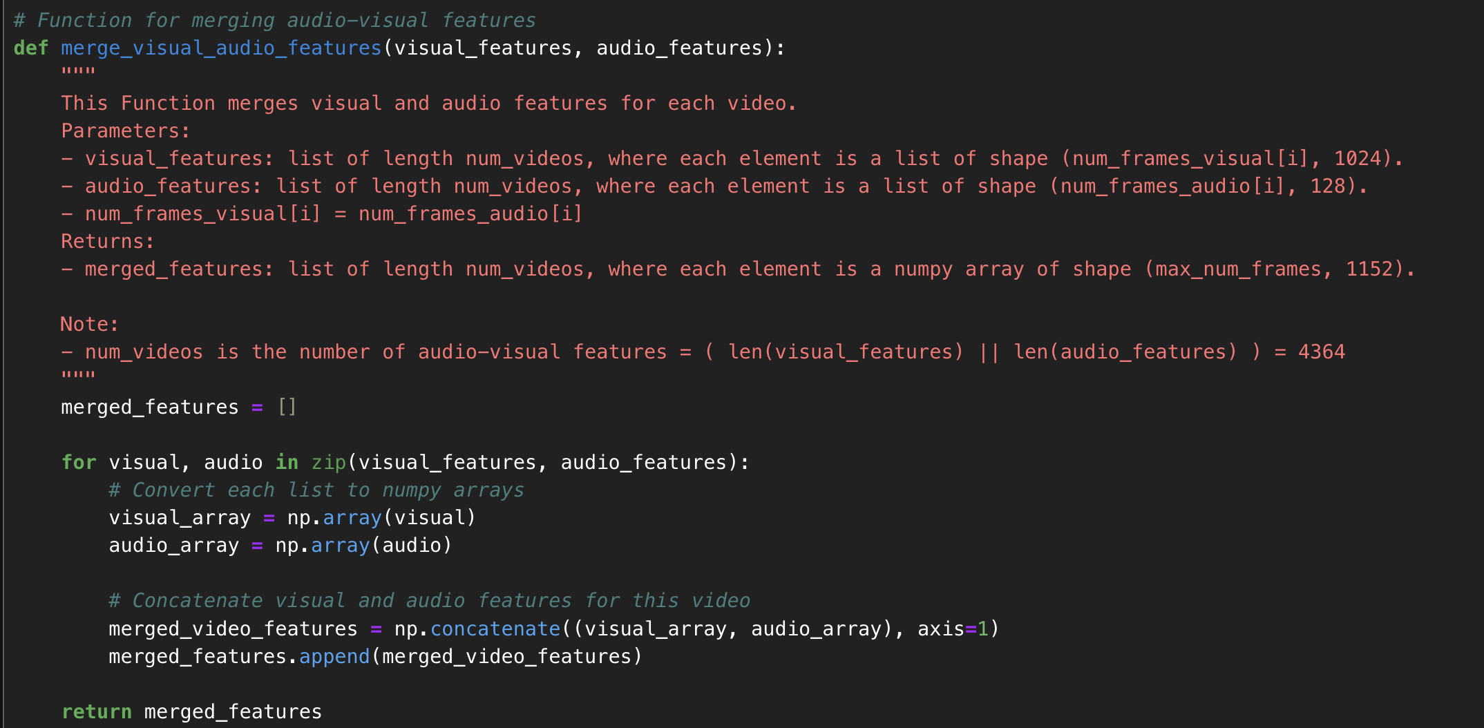This function gave an output with dimensions:

commercialFeatures: [4364][119-300][1152]
nonCommercialFeatures: [4600][109-301][1152]

Why 1152?

Audio + Visual Features = 128 + 1024 = 1152

Generating Uniform Features

Now, the next task is to convert these features into an ndarray. However, this is not possible unless the features are uniform.

In our case, the second dimension of the features is not uniform. So, we need to either pad or trim the features to a definite sequence length. Which sequence length would be best for model training? It’s not possible to say without testing.

Data Visualization

Let’s Visualize the data first:

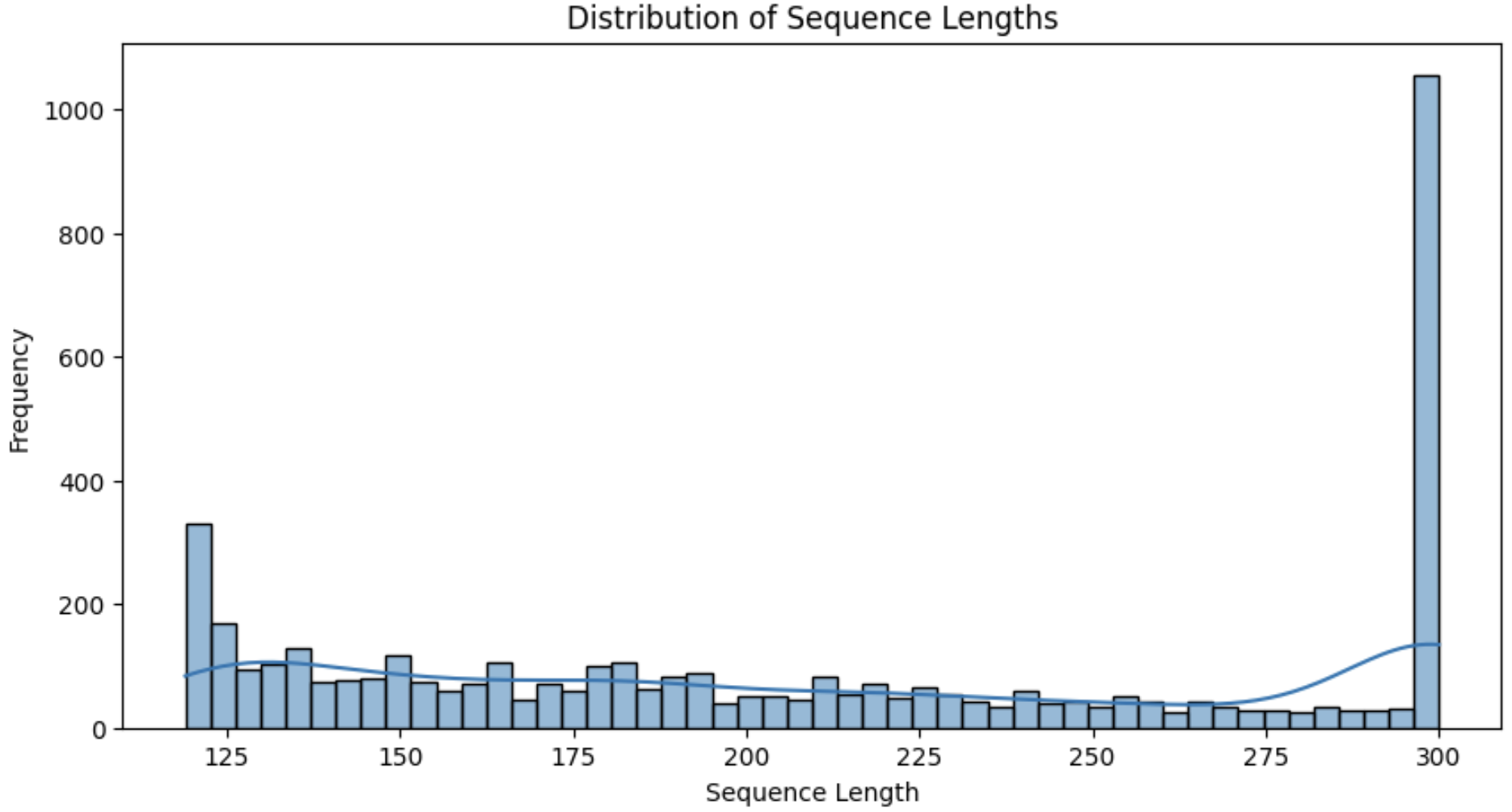
commercialFeatures:

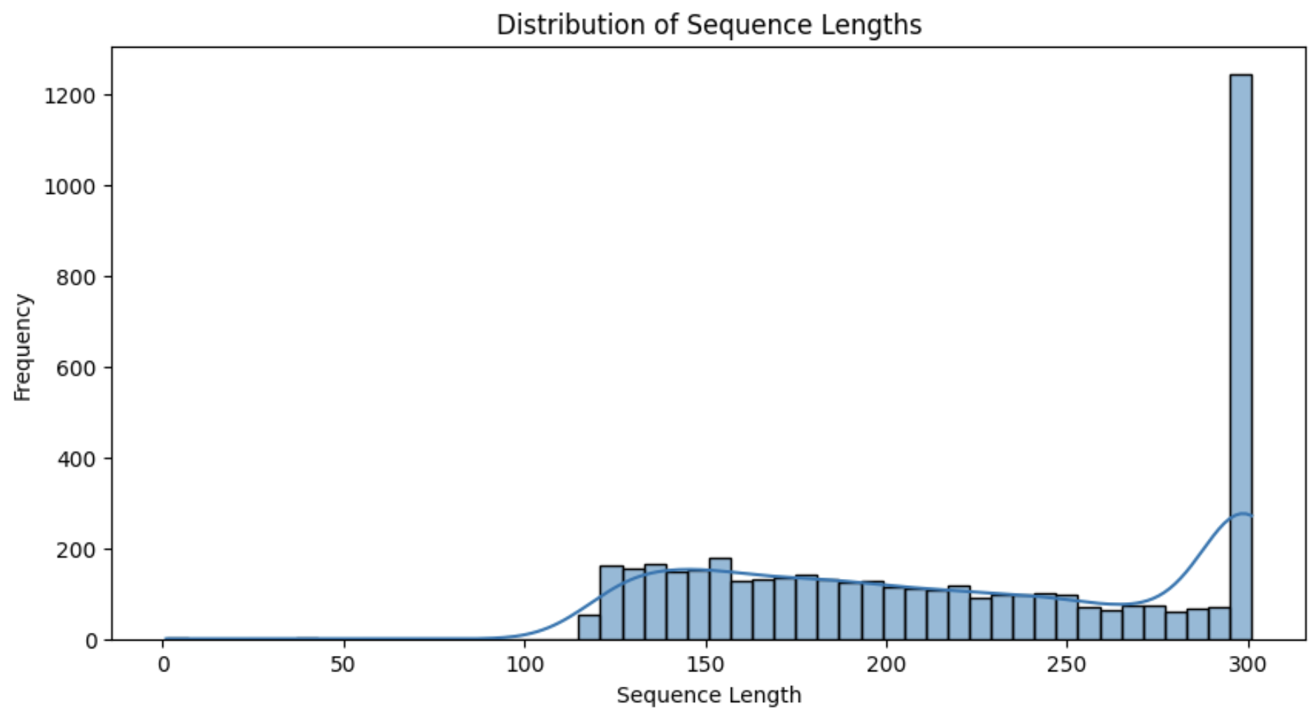
nonCommercialFeatures:

Analysis of commercialFeatures:

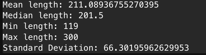
Analysis of nonCommercialFeatures

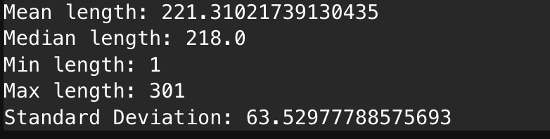
The frequency of a few sequence length frames in commercialFeatures is shown below (not sharing frequencies of all the frames, as it would be unnecessary and very large):

Sequence_length: 282, Frequency: 14
Sequence_length: 283, Frequency: 4
Sequence_length: 284, Frequency: 3
Sequence_length: 285, Frequency: 13
Sequence_length: 286, Frequency: 7
Sequence_length: 287, Frequency: 8
Sequence_length: 288, Frequency: 8
Sequence_length: 289, Frequency: 6
Sequence_length: 290, Frequency: 6
Sequence_length: 291, Frequency: 12
Sequence_length: 292, Frequency: 11
Sequence_length: 293, Frequency: 10
Sequence_length: 294, Frequency: 9
Sequence_length: 295, Frequency: 5
Sequence_length: 296, Frequency: 7
Sequence_length: 297, Frequency: 11
Sequence_length: 298, Frequency: 10
Sequence_length: 299, Frequency: 12
Sequence_length: 300, Frequency: 1022

Padding or Trimming what to do?

Padding involves adding extra values (usually zeros) to sequences so that all sequences in a batch have the same length, whereas trimming involves cutting sequences to a maximum length, either by removing elements from the beginning, end, or middle of the sequence. The choice between padding and trimming depends on the specific requirements of the task and the model being used. Striking the right balance between maintaining relevant information and ensuring computational efficiency is key to optimizing model performance.

So, I have decided to test out different sequence lengths for model training and go with the one which gives the maximum accuracy. The different sequence lengths I will try to train the model with are 150, 200, and 300.

The following code generates the padded/trimmed uniform features and then converts them into an ndarray:

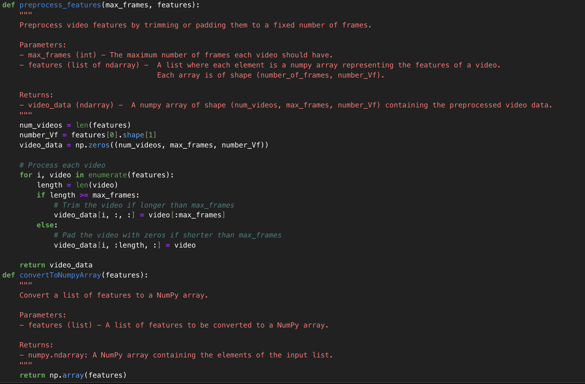
This generates a NumPy array of dimensions [len(features)][max_frames][1152]

Generating Labels for Data and Merging Commercial and Non-Commercial Features, and Shuffling Data Randomly

Labels are generated corresponding to both features: 1 for commercial video features and 0 for non-commercial video features. The features are then shuffled in unison with labels to create random data.

Afterwards, the data is scaled between 0 and 1, and standardized to ensure that each feature contributes equally to the model’s performance, avoiding bias toward features with larger scales.

Following the train, test, and validation split of data in the ratio 7:1.5:1.5 respectively, the data is now ready to be fed into a machine learning model.

Thank you for reading the blog. Happy coding, peers!

The upcoming blog will focus on the model training process and its results.

Links:

Link to model preprocessing and ongoing model pipeline preparation code: Link

← Previous Post Next Post →

Dataset PreProcessing

Week 3-4